# (C) WiSi-Testpilot, letzte Anderung: 11.5.2023
# cd C:\Users\Wilsi\Desktop\k3
import glob
import time
import math as m
import random
import datetime
import numpy as np
import cv2
import pixellib
import tensorflow as tf
from shapely.geometry import Polygon
startzeit = datetime.datetime.now()
print("#### Num GPUs Available: ", len(tf.config.list_physical_devices('GPU')))
from pixellib.instance import custom_segmentation
segment_image = custom_segmentation()
segment_image.inferConfig(num_classes= 3, class_names= ["BG", "Artifical-Star", "Background", "Meteor"])
segment_image.load_model("C:/Users/Wilsi/Desktop/k3/drei-Klassen/mask_rcnn_model.040-0.432872.h5")
sname = " mask_rcnn_model.040-0.432872, Filter 550/1000 "
debug = 1
# 0: normal, batch
# 1: Stop bei Echo,
# 2: Stop bei Score unter 0.8,
# 3: Stop bei Starlink,
# 4: Stop bei Echo > 10000
# 5: Stop bei jedem Plot, also auch bei leeren Bilden
# 6: Stop bei dopplershift > 550 and summe < 1000 # 550 und 1000 sind Parameter
Aufnahmejahr = " 2023,"
path = glob.glob("C:/Users/Wilsi/Desktop/mai11/GRAVES-xymVV_230512*.jpg") # normale wildcard-Regeln
#path = glob.glob("C:/Users/Willi/Desktop/Met-Mai22XY-1-31/GRAVES-XY-Vv_220505*.jpg")
#path = glob.glob("C:/Users/Wilsi/Desktop/Juni22-8-10/GRAVES-XY-Vv_220609102*.jpg")
#path = glob.glob("C:/Users/Willi/Desktop/2022-Dez13-15/GRAVES-xy_221214*.jpg")
#path = glob.glob("C:/Users/Willi/Desktop/DezXY12-24/GRAVES-XY-Vv_211214*.jpg")
#path = glob.glob("C:/Users/Willi/Desktop/Jan3-6-23/GRAVES-xy_230104*.jpg")
bg = np.zeros((550, 1900, 3), np.uint8) # Output Display
summe_3min = np.zeros((481), np.uint32)
fsumme_3min = np.zeros((481), np.single)
su1 = np.zeros((481), np.uint32)
su2 = np.zeros((481), np.uint32)
su3 = np.zeros((481), np.uint32)
su4 = np.zeros((481), np.uint32)
su5 = np.zeros((481), np.uint32)
su6 = np.zeros((481), np.uint32)
histogramm = np.zeros((540, 510, 3), np.uint8) #Histogramm Display
summe_fl = np.zeros((26), np.single)
summe_anz = np.zeros((26), np.uint32)
summe_anz_Starlink = np.zeros((26), np.uint32)
score_100_99 = 0
score_99_98 = 0
score_98_97 = 0
score_97_96 = 0
score_96_95 = 0
score_95_94 = 0
score_94_93 = 0
score_93_90 = 0
score_90_80 = 0
score_80_70 = 0
score_70_00 = 0
Baseline = 700
kleiner_Baseline = 0
kleiner_Baseline_alle = 0
plot_count = 0
globalcount = 0
Art_count = 0
BG_count = 0
Err_count = 0
noisefloor = 1
fontScale = 0.6
fthickness = 1
font = cv2.FONT_HERSHEY_SIMPLEX
RED = (0, 0, 255) # b g r
GREEN = (20, 255, 20,)
YELLOW = (0, 255, 255)
BLUE = (255, 0, 0)
Magenta = (147, 20, 255)
DarkOrange = (15, 185, 255) # Gold
WHITE = (200, 200, 200)
Gray = (100, 100, 100)
light_BLUE = (255, 191, 0)
DarkOrange1 = (0, 140, 255) # alt
lite_MAGENTA = (255, 0, 255)
Rose = (200, 200, 255)
lRED = (20, 20, 200) # b g r
OrangeRed = (0, 190, 255) # b g r fast gelb
darkOlive = (40, 120, 40)
Olive = (150, 255, 150)
for fname in path: # Analyse über alle Files im Ordner/Folder
print(' > ', fname)
position = fname.find(".jpg") # Zeit und Datum werden aus dem Filenamen extrahiert
zeit = fname[position-10:position]
print ("Jahr Monat Tag St. Min. Sek.", '20' + fname[position-12:position])
monat= zeit[0:2]
if monat == '01': Monat = 'Januar'
if monat == '02': Monat = 'Februar'
if monat == '03': Monat = 'Maerz'
if monat == '04': Monat = 'April'
if monat == '05': Monat = 'Mai'
if monat == '06': Monat = 'Juni'
if monat == '07': Monat = 'Juli'
if monat == '08': Monat = 'August'
if monat == '09': Monat = 'September'
if monat == '10': Monat = 'Oktober'
if monat == '11': Monat = 'November'
if monat == '12': Monat = 'Dezember'
day= zeit[2:4]
ho = zeit[4:6] # Zeit aus Filenamen extrahieren
mi = zeit[6:8]
se = zeit[8:10]
# print('Monat: ', monat)
# print('Tag: ', day)
# print (day + '.', Monat, '2023')
ctime = (float(ho) * 3600 ) + (float(mi) *60) + float(se) # X-Position aus Zeit berechnen
# print('################# ctime ', round(ctime), ' ', round(ctime/20), ' ', round(ctime/180))
xa = round (ctime / 60)
if (mi == '00') and ((se == '00') or (se == '59') or (se == '01') ):
bg = cv2.line(bg,(xa,500),(xa, 515), WHITE, 2) # X ganze Stunden-Ticks
org = (xa, 530) # war 535
bg = cv2.putText(bg, ho, org, font, fontScale, WHITE, fthickness, cv2.LINE_AA)
if ((mi == '30') or (mi == '15') or (mi == '45')) and ((se == '00') or (se == '59') or (se == '01') ):
bg = cv2.line(bg,(xa,500),(xa, 510), WHITE, 1) # X 1/4 Stunden-Ticks
isClosed = True
dicke = 3
radius = 4
org = (0, 0)
meteor_was_there = False # Debug
klein_meteor_was_there = False
starlink_was_there = False
ue10000_was_there = False
traeger_was_there = False
paare = np.zeros((1000,2), np.int32)
bg_RED = np.zeros((1000,2), np.int32)
bg_GREEN = np.zeros((1000,2), np.int32)
bg_YELLOW = np.zeros((1000,2), np.int32)
bg_BLUE = np.zeros((1000,2), np.int32)
bg_Magenta = np.zeros((1000,2), np.int32)
bg_DarkOrange = np.zeros((1000,2), np.int32)
bg_WHITE = np.zeros((1000,2), np.int32)
bg_light_BLUE = np.zeros((1000,2), np.int32)
bg_DarkOrange1 = np.zeros((1000,2), np.int32)
bg_lite_MAGENTA = np.zeros((1000,2), np.int32)
bg_Rose = np.zeros((1000,2), np.int32)
bg_lRED = np.zeros((1000,2), np.int32)
bg_OrangeRed = np.zeros((1000,2), np.int32)
bg_darkOlive = np.zeros((1000,2), np.int32)
bg_Olive = np.zeros((1000,2), np.int32)
summe_RED = 0
summe_GREEN = 0
summe_YELLOW = 0
summe_BLUE = 0
summe_Magenta = 0
summe_DarkOrange = 0
summe_WHITE = 0
summe_light_BLUE = 0
summe_DarkOrange1 = 0
summe_lite_MAGENTA = 0
summe_Rose = 0
summe_lRED = 0
summe_OrangeRed = 0
summe_darkOlive = 0
summe_Olive = 0
anz_RED = 0
anz_GREEN = 0
anz_YELLOW = 0
anz_BLUE = 0
anz_Magenta = 0
anz_DarkOrange = 0
anz_WHITE = 0
anz_light_BLUE = 0
anz_DarkOrange1 = 0
anz_lite_MAGENTA = 0
anz_Rose = 0
anz_lRED = 0
anz_OrangeRed = 0
anz_darkOlive = 0
anz_Olive = 0
# Bild wird analysiert
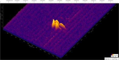
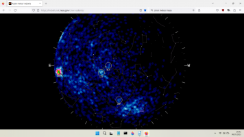
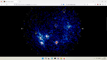
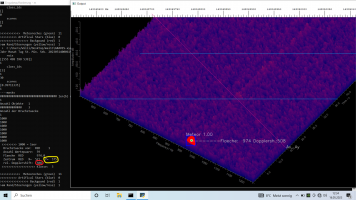
segmask, output = segment_image.segmentImage (fname, mask_points_values=True, show_bboxes=True) #, output_image_name="2-testy.jpg")
print (' rois')
a = segmask.get('rois')
print (a)
print (len(a))
print (' class_ids')
# Noise Floor auswerten
if len(a) == 0:
nfmittelwert = 0.0
if noisefloor == 1:
for i_nf in range (300, 401):
for j_nf in range (200, 301):
for k_nf in range (0, 3):
nfmittelwert = nfmittelwert + output[i_nf, j_nf, k_nf]
cv2.circle(bg, (xa, 500 - int(nfmittelwert/5000)), 1 , Magenta, -1)
# Debugg Noisefloor
# print (nfmittelwert/5000)
# cv2.rectangle(output, (300, 200), (400, 300), YELLOW, 2)
# cv2.imshow("Bild fuer NF", output)
# cv2.waitKey(0)
# cv2.destroyAllWindows()
#b = segmask.get('class_ids')
b = segmask['class_ids'].astype('int')
print (b)
print (len(b))
test = np.zeros((100), np.int32)
for itest in range (0, len(b)):
test[itest] = b[itest]
print (test[itest]*10)
print (' scores')
c = segmask.get('scores')
print (c)
print (len(c))
if len(c) > 0:
print ('----masks')
if len(b) > 1: d = segmask.get('masks')
if len(b) == 1:
try:
d = segmask['masks'].astype('int')
print ('################################## len(b) war 1 ')
except:
d = segmask.get('masks')
# print('*********')
print (len(d))
# print(d)
anzahl = 0
anzahl = len(d)
print ('Anzahl Objekte ', anzahl)
####### Konturen werden ausgewertet
counter = 0
color = Olive
# for i in d: cv2.polylines(output, i, isClosed, light_BLUE, dicke)
for i in d:
counter += 1
print('############# ', b[counter -1])
if counter == 1:
color = RED
bg_RED = i
if counter == 2:
color = GREEN
bg_GREEN = i
if counter == 3:
color = YELLOW
bg_YELLOW = i
if counter == 4:
color = BLUE
bg_BLUE = i
if counter == 5:
color = Magenta
bg_Magenta = i
if counter == 6:
color = DarkOrange
bg_DarkOrange = i
if counter == 7:
color = WHITE
bg_WHITE = i
if counter == 8:
color = light_BLUE
bg_light_BLUE = i
if counter == 9:
color = DarkOrange1
bg_DarkOrange1 = i
if counter == 10:
color = lite_MAGENTA
bg_lite_MAGENTA = i
if counter == 11:
color = Rose
bg_Rose = i
if counter == 12:
color = lRED
bg_lRED = i
if counter == 13:
color = OrangeRed
bg_OrangeRed = i
if counter == 14:
color = darkOlive
bg_darkOlive = i
if counter == 15:
color = Olive
bg_Olive = i
print('Anzahl der Bruchstuecke ')
print(len(bg_RED))
print(len(bg_GREEN))
print(len(bg_YELLOW))
print(len(bg_BLUE))
print(len(bg_Magenta))
print(len(bg_DarkOrange))
print(len(bg_WHITE))
print(len(bg_light_BLUE))
# hier fehlt noch 9-15
print(' >>>>>>>>> 1000 = leer')
for o in range (1, anzahl +1):
if o == 1:
bg_temp = bg_RED
col_temp = RED
col_name = 'RED'
if o == 2:
bg_temp = bg_GREEN
col_temp = GREEN
col_name = 'GREEN'
if o == 3:
bg_temp = bg_YELLOW
col_temp = YELLOW
col_name = 'YELLOW'
if o == 4:
bg_temp = bg_BLUE
col_temp = BLUE
col_name = 'BLUE'
if o == 5:
bg_temp = bg_Magenta
col_temp = Magenta
col_name = 'Magenta'
if o == 6:
bg_temp = bg_DarkOrange
col_temp = DarkOrange
col_name = 'DarkOrange'
if o == 7:
bg_temp = bg_WHITE
col_temp = WHITE
col_name = 'WHITE'
########### hier fehlt noch 8-15
# if test[o-1] > 1: cv2.fillPoly(output, bg_temp, col_temp)
laenge = len(bg_temp)
print (' Bruchstuecke von: ', col_name, ' ', laenge)
counter = 0
summe = 0
xsumme = 0
ysumme = 0
for ii in bg_temp:
print (' Anzahl Wertepaare: ', len(ii))
paare = np.zeros((len(ii),2), np.int32)
if len(ii) >= 3:
counter = 0
for jj in ii:
paare[counter] = jj
counter += 1
cv2.fillPoly(output, [paare], col_temp)
pgon = Polygon(paare)
summe += pgon.area
print (' Flaeche ', col_name, ' ', pgon.area)
mitte_x = round(pgon.centroid.x)
xsumme += mitte_x
mitte_y = round(pgon.centroid.y)
ysumme += mitte_y
print (' Zentrum ', col_name, ' X= ', mitte_x, ' Y= ', mitte_y)
if len(ii) < 3:
print (' >>>>>>>>>>>>>>>>>>>>>>>>>>>>>>>>>>>>>>>>>verworfen ')
laenge -= 1
if laenge > 1:
print (' >>>>>> Mittelwert Zentrum: ', col_name, ' Xs= ', round(xsumme / laenge), ' Ys= ', round(ysumme / laenge))
print (' >>>>>>>> Summe der Fläche: ', summe)
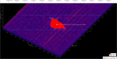
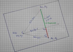
########### Dopplershift berechnen
if laenge > 0:
org = (round(xsumme / laenge), round(ysumme / laenge))
Ax = 930 # Projektionslini für die Dopplerschift.
Ay = 609
Bx = 350
By = 28
cv2.line(output, (Ax, Ay),(Bx, By), Magenta, 1)
cv2.putText(output, ('Ax, Ay'), (Ax, Ay), font, fontScale, WHITE, fthickness, cv2.LINE_AA)
dx = Bx - Ax
dy = By - Ay
cqu = dx*dx + dy*dy
c_geo = m.sqrt(cqu)
# print (' c_geo ', c_geo)
ux, uy = org
dx = Bx - ux
dy = By - uy
a1_geo = m.sqrt(dx*dx + dy*dy)
# print (' a1_geo ',a1_geo)
dx = Ax - ux
dy = Ay - uy
b1_geo = m.sqrt(dx*dx + dy*dy)
# print (' b1_geo ',b1_geo)
try:
cos_alpha = (b1_geo * b1_geo + cqu - a1_geo * a1_geo)/(2*b1_geo * c_geo) #Cosinussatz
except:
cos_alpha = 0.7
# print (' cos alpha ', cos_alpha)
try:
A_arc = m.acos(cos_alpha)
except:
A_arc = 99
sin_A = m.sin(A_arc)
cos_A = m.cos(A_arc)
A_deg = np.rad2deg(A_arc)
# print (' Alpha ',A_deg)
hoehe1 = b1_geo * sin_A
# print (' Hoehe: ', hoehe1)
dopplershift = round (m.sqrt(a1_geo * a1_geo - hoehe1 * hoehe1))
print (' rel. Dopplershift: ', dopplershift)
############### Ende Dopplershift
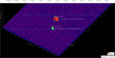
print (' >>>>>>>>>>>>>>>>>>>> Klasse: ', test[o-1])
cv2.circle(output, org, 6 , WHITE, -1)
if col_name == 'RED': cv2.circle(output, org, 3 , GREEN, -1)
if col_name != 'RED': cv2.circle(output, org, 3 , RED, -1)
fsize = ("{:5.0f}".format(summe))
ds = ("{:3.0f}".format(dopplershift))
############ Flags fuer debug
if test[o-1] == 1: starlink_was_there = True
if test[o-1] == 3: meteor_was_there = True
if c[o-1] < 0.8: klein_meteor_was_there = True
if test[o-1] == 3 and summe > 10000: ue10000_was_there = True
if (test[o-1] == 3) and (dopplershift > 550 and summe < 1000): traeger_was_there = True
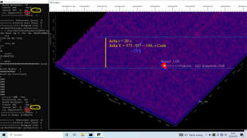
############ Echos im Bereich 200 bis 396 loggen. 196 (200 bis 396) entspricht 20 Sekunden in meinen Plots.
############ Ausser bei der Dopplershift ist dies der einzige Parameter. Den Wert kann man im Einzelschrittmodus ablesen.
if (uy >= 200) and ( uy < 396) and (test[o-1] == 3) and (dopplershift > 300) and (dopplershift < 700) and (summe < 100000) and not \
(dopplershift > 550 and summe < 1000): # Stoerung siehe todo Doku
fontScale = 0.6
fsize = '++++++Flaeche:' + fsize + ' Dopplersh.:' + ds
print (' Score in Window ', c[o-1])
if (c[o-1] <= 1.00) and (c[o-1] > 0.99): score_100_99 += 1
if (c[o-1] <= 0.99) and (c[o-1] > 0.98): score_99_98 += 1
if (c[o-1] <= 0.98) and (c[o-1] > 0.97): score_98_97 += 1
if (c[o-1] <= 0.97) and (c[o-1] > 0.96): score_97_96 += 1
if (c[o-1] <= 0.96) and (c[o-1] > 0.95): score_96_95 += 1
if (c[o-1] <= 0.95) and (c[o-1] > 0.94): score_95_94 += 1
if (c[o-1] <= 0.94) and (c[o-1] > 0.93): score_94_93 += 1
if (c[o-1] <= 0.93) and (c[o-1] > 0.90): score_93_90 += 1
if (c[o-1] <= 0.90) and (c[o-1] > 0.80): score_90_80 += 1
if (c[o-1] <= 0.80) and (c[o-1] > 0.72): score_80_70 += 1
if (c[o-1] <= 0.72) and (c[o-1] > 0.00): score_70_00 += 1
offset_summe = summe - Baseline
if offset_summe <= 0:
offset_summe = 1
kleiner_Baseline_alle +=1
if (c[o-1] >= 0.72): # nur hier loggen
y_t_color = GREEN
if offset_summe == 1: kleiner_Baseline += 1
fl = int(495 -100 * m.log10(offset_summe))
globalcount += 1
bg = cv2.circle(bg, (xa, fl), dicke , y_t_color, -1)
###### 1800 für 30 Minuten oder 2 Werte pro Stunde
# ! # 720 für 12 Minuten oder 5 Werte pro Stunde
# ! # 360 für 6 Minuten oder 10 Werte pro Stunde
####### 180 für 3 Minuten oder 20 Werte pro Stunde
plot_count = m.trunc(ctime / 1800)
summe_3min[plot_count] += 1
fsumme_3min[plot_count] = fsumme_3min[plot_count] + summe
if (summe > 0) and (summe < 500): su1[plot_count] += 1
if (summe >= 500) and (summe < 1000): su2[plot_count] += 1
if (summe >= 1000) and (summe < 3000): su3[plot_count] += 1
if (summe >= 3000) and (summe < 10000): su4[plot_count] += 1
if (summe >= 10000) and (summe < 100000): su5[plot_count] += 1
if (c[o-1] >= 0.98): su6[plot_count] += 1 # score 0.98
summe_anz[int(ho)+1] +=1
summe_fl[int(ho)+1] = summe_fl[int(ho)+1] + summe
################ Störung "Träger" innerhalb der 20 Sekunden
if (uy >= 200) and ( uy < 396) and (dopplershift > 550 and summe < 1000):
fontScale = 0.6
fsize = '-x-T-x--Flaeche:' + fsize + ' Dopplersh.:' + ds
y_t_color = Rose
Err_count += 1
offset_summe = summe - Baseline
if offset_summe <= 0: offset_summe = 1
fl = int(495 -100 * m.log10(summe))
bg = cv2.circle(bg, (xa, fl), dicke , y_t_color, -1)
################ Echos liegen zu nahe am Rand
if (uy >= 200) and ( uy < 396) and (test[o-1] == 3) and ((dopplershift <= 300) or (dopplershift >= 700)):
fontScale = 0.6
fsize = '-x-W-x--Flaeche:' + fsize + ' Dopplersh.:' + ds
y_t_color = YELLOW
Err_count += 1
offset_summe = summe - Baseline
if offset_summe <= 0: offset_summe = 1
fl = int(495 -100 * m.log10(summe))
bg = cv2.circle(bg, (xa, fl), dicke , y_t_color, -1)
################ Background innerhalb der 20 Sekunden loggen
if (uy >= 200) and ( uy < 396) and (test[o-1] == 2) and (dopplershift >= 20): # Rand weg
fontScale = 0.6
fsize = '----R---Flaeche:' + fsize + ' Dopplersh.:' + ds
y_t_color = RED
BG_count += 1
offset_summe = summe - Baseline
if offset_summe <= 0: offset_summe = 1
fl = int(495 -100 * m.log10(offset_summe))
bg = cv2.circle(bg, (xa, fl), 2 , y_t_color, -1) # 2 = dicke
################ Starlinks innerhalb der 20 Sekunden loggen
if (uy >= 200) and ( uy < 396) and (test[o-1] == 1) and (c[o-1] >= 0.0):
fontScale = 0.6
fsize = '----B----Flaeche:' + fsize + ' Dopplersh.:' + ds
y_t_color = BLUE
Art_count += 1
offset_summe = summe - Baseline
if offset_summe <= 0: offset_summe = 1
fl = int(495 -100 * m.log10(offset_summe))
bg = cv2.circle(bg, (xa, fl), dicke , y_t_color, -1)
summe_anz_Starlink[int(ho)+1] +=1
################ Rest ausserhalb der 20 Sekunden beschriften
if (uy < 200) or ( uy >= 396): #196
fontScale = 0.6
fsize = '--------Flaeche:' + fsize + ' Dopplersh.:' + ds
ux, uy = org
uy += 8
cv2.putText(output, fsize, (ux, uy), font, fontScale, WHITE, fthickness, cv2.LINE_AA)
fontScale = 0.6
#### Auswertebereich einzeichnen. 196 (200 bis 396) entspricht 20 Sekunden in meinen Plots.
#### Ausser bei der Dopplershift ist dies der einzige Parameter. Den Wert kann man im Einzelschrittmodus ablesen.
Ax1 = 300
Ay1 = 200
Bx1 = 1350
By1 = 200
cv2.line(output, (Ax1, Ay1),(Bx1, By1), light_BLUE, 1)
Ax2 = 100
Ay2 = 200 + 196
Bx2 = 1150
By2 = 200 + 196
cv2.line(output, (Ax2, Ay2),(Bx2, By2), light_BLUE, 1)
print ()
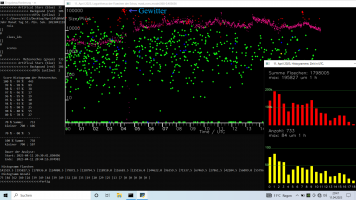
print ('>>>>>>>>>>>> Meteorechos (green) ', globalcount)
print ('>>>>>>>>>> Artifical Stars (blue) ', Art_count)
print ('>>>>>>>>>>>>>>>>> Backgound (red) ', BG_count)
print ('>am Rand/Stoerungen (yellow/rose) ', Err_count)
if (debug == 1 and meteor_was_there == True) or ( debug == 2 and klein_meteor_was_there == True) or \
(debug == 3 and starlink_was_there == True) or ( debug == 4 and ue10000_was_there == True) or debug == 5 or (debug == 6 and traeger_was_there == True):
cv2.imwrite("output.png", output)
cv2.imshow("Output", output)
cv2.waitKey(0)
stream = cv2.imread(fname)
cv2.imshow("Output", stream)
cv2.imwrite("input.png", stream)
cv2.waitKey(0) #################
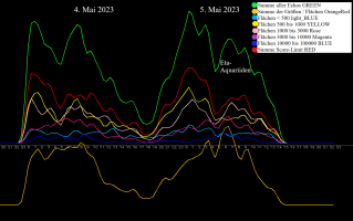
cv2.line(bg,(1,1),(1,500),(WHITE),2)
cv2.line(bg,(1,499),(1900,499), WHITE,2) # Skala
for grj in range (1,5):
bg = cv2.line(bg,(0, grj * 100),(15, grj * 100), WHITE,2) # Y- Ticks
off = 4
cv2.putText(bg, '1', (5, 500-off), font, fontScale, WHITE, fthickness, cv2.LINE_AA)
cv2.putText(bg, '10', (5, 400-off), font, fontScale, WHITE, fthickness, cv2.LINE_AA)
cv2.putText(bg, '100', (5, 300-off), font, fontScale, WHITE, fthickness, cv2.LINE_AA)
cv2.putText(bg, '1000', (5, 200-off), font, fontScale, WHITE, fthickness, cv2.LINE_AA)
cv2.putText(bg, '10000', (5, 100-off), font, fontScale, WHITE, fthickness, cv2.LINE_AA)
cv2.putText(bg, '100000', (5, 20), font, fontScale, WHITE, fthickness, cv2.LINE_AA)
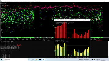
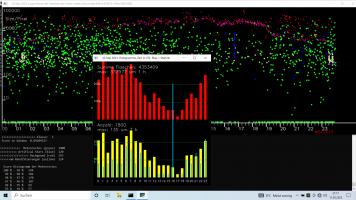
cv2.putText(bg, 'Size/Pixel', (15, 55), font, fontScale, WHITE, fthickness, cv2.LINE_AA)
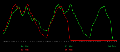
cv2.putText(bg,'Time / UTC', (580, 543), font, fontScale, WHITE, fthickness, cv2.LINE_AA)
cv2.putText(bg,'WiSi 2023', (1350,543), font, 0.5, RED, fthickness, cv2.LINE_AA)
cv2.imshow(' ' + day +'. ' + Monat + Aufnahmejahr +' Logarithmus der Flaechen der Echos,' + sname, bg)
cv2.imwrite("bg.png", bg)
isscore = score_100_99 + score_99_98 +score_98_97 + score_97_96 + score_96_95 + score_95_94 + score_94_93 + score_93_90 + score_90_80 + score_80_70
sscore = score_100_99 + score_99_98 +score_98_97 + score_97_96 + score_96_95 + score_95_94 + score_94_93 + score_93_90 + score_90_80 + score_80_70 + score_70_00
print()
print (' Score Histogramm der Meteorechos')
print (' 100 % - 99 % ', score_100_99)
print (' 99 % - 98 % ', score_99_98)
print (' 98 % - 97 % ', score_98_97)
print (' 97 % - 96 % ', score_97_96)
print (' 96 % - 95 % ', score_96_95)
print (' 95 % - 94 % ', score_95_94)
print (' 94 % - 93 % ', score_94_93)
print (' 93 % - 90 % ', score_93_90)
print (' 90 % - 80 % ', score_90_80)
print (' 80 % - 70 % ', score_80_70)
print ('------------------------')
print (' 70 % Summe: ', isscore)
print (' kleiner ', Baseline, ':', kleiner_Baseline)
print()
print (' 70 % - 00 % ', score_70_00)
print ('------------------------')
print (' 100 % Summe: ', sscore)
print (' kleiner ', Baseline, ':', kleiner_Baseline_alle)
print ()
print (' Dauer der Analyse: ')
print (' Start:',startzeit)
now = datetime.datetime.now()
print (' Ende: ', now)
print ()
sugesamt = isscore
fl_max = 0
fl_max_i = 0
fl_sum = 0
print (' Histogramm Flaechen ')
for ihis in range (1,25):
fl_sum = fl_sum + summe_fl[ihis]
if fl_max < summe_fl[ihis]:
fl_max = summe_fl[ihis]
fl_max_i = ihis
print (summe_fl[ihis], end = ' |')
print ( '', end = "\r\n")
anz_max = 0
anz_max_i = 0
print (' Histogramm Anzahl ')
for ihis in range (1,25):
if anz_max < summe_anz[ihis]:
anz_max = summe_anz[ihis]
anz_max_i = ihis
print (summe_anz[ihis], end = ' |')
print ( '', end = "\r\n")
fontScale1 = 0.4
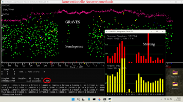
for ihis in range (1,25):
cv2.rectangle(histogramm, (ihis*20, 250), ((ihis * 20) +10, 250 - int(summe_fl[ihis]/333.33/4)), RED, -1)
cv2.rectangle(histogramm, (ihis*20, 500), ((ihis * 20) +10, 500 - summe_anz[ihis]*3//2), YELLOW, -1)
cv2.rectangle(histogramm, (ihis*20 +4, 500), ((ihis * 20) + 6, 500 - summe_anz_Starlink[ihis]*30//2), light_BLUE, -1) # Starlink
org = (int(ihis*19.9), 520)
cv2.putText(histogramm, str(ihis-1), org, font, fontScale1, WHITE, fthickness, cv2.LINE_AA)
# 250 -75 -75
cv2.line(histogramm,(30, 175),(490, 175), darkOlive, 1)
cv2.line(histogramm,(30, 100),(490, 100), darkOlive, 1)
cv2.putText(histogramm, '100k', (4, 175), font, fontScale1, Olive, fthickness, cv2.LINE_AA)
cv2.putText(histogramm, '200k',(4, 100), font, fontScale1, Olive, fthickness, cv2.LINE_AA)
# 500 -75 -75
cv2.line(histogramm,(20, 425),(490, 425), darkOlive, 1)
cv2.line(histogramm,(20, 350),(490, 350), darkOlive, 1)
cv2.putText(histogramm, '50', (4, 425), font, fontScale1, Olive, fthickness, cv2.LINE_AA)
cv2.putText(histogramm, '5', (4, 438), font, fontScale1, light_BLUE, fthickness, cv2.LINE_AA)
cv2.putText(histogramm, '100', (4, 350), font, fontScale1, Olive, fthickness, cv2.LINE_AA)
cv2.putText(histogramm, '10', (4, 363), font, fontScale1, light_BLUE, fthickness, cv2.LINE_AA)
cv2.putText(histogramm, ' Summe Flaechen: '+str(int(fl_sum)), (10, 30), font, fontScale, WHITE, fthickness, cv2.LINE_AA)
cv2.putText(histogramm, ' max: '+ str(int(fl_max)) + ' um '+ str(fl_max_i - 1)+ ' h', (10, 50), font, fontScale, WHITE, fthickness, cv2.LINE_AA)
cv2.putText(histogramm, ' Anzahl: '+str(int(sugesamt)), (10, 280), font, fontScale, WHITE, fthickness, cv2.LINE_AA)
cv2.putText(histogramm, ' max: '+str(anz_max) + ' um ' + str(anz_max_i - 1) + ' h', (10, 300), font, fontScale, WHITE, fthickness, cv2.LINE_AA)
cv2.imshow(' ' + day +'. ' + Monat +' 2023, Histogramme, Zeit in UTC, Blau = Starlink', histogramm)
with open('datum.txt', 'w') as f:
f.write(' Aufnahme ' + day + '. '+ Monat + ' 2023' + sname + '\n')
f.write(' Zeit Anzahl Flaeche 500 1000 3000 10000 100000 Score 0.98' + '\n')
for out_count in range (0, 48): # 48 für 30 Minuten, 120 für 12 Minuten, 240 für 6 Minuten, 480 für 3 Minuten
out_i = ("{:6.0f}".format(out_count//(2))) # 2 für 30 Minuten, 5 für 12 Minuten, 10 für 6 Minuten, 20 für 3 Minuten
outn = ("{:8.0f}".format(summe_3min[out_count]))
outf = ("{:8.0f}".format(round(fsumme_3min[out_count])))
out1 = ("{:8.0f}".format(su1[out_count]))
out2 = ("{:8.0f}".format(su2[out_count]))
out3 = ("{:8.0f}".format(su3[out_count]))
out4 = ("{:8.0f}".format(su4[out_count]))
out5 = ("{:8.0f}".format(su5[out_count]))
out6 = ("{:8.0f}".format(su6[out_count]))
f.write(' UTC' + out_i + outn + outf + out1 + out2 + out3 + out4 + out5 + out6 + ' \n')
f.write('\r\n')
with open('alt-datum.txt', 'w') as f:
for out_count in range (0, 48): # 48 für 30 Minuten, 120 für 12 Minuten, 240 für 6 Minuten, 480 für 3 Minuten
susi_i = ("{:8.0f}".format(out_count//(2))) # 2 für 30 Minuten, 5 für 12 Minuten, 10 für 6 Minuten, 20 für 3 Minuten
susi_3min = ("{:8.0f}".format(round(summe_3min[out_count]/1)))
if out_count > 0: f.write(' ' + susi_i + susi_3min + ' \n')
if out_count == 0: f.write(' ' + susi_i + susi_3min + ' Aufnahme ' + day + '. '+ Monat + ' 2023' + sname + '\n')
f.write('\r\n')
for out_count in range (0, 240):
susi_i = ("{:8.0f}".format(out_count//(10)))
susi_3min = ("{:8.0f}".format(round(fsumme_3min[out_count]/1)))
if out_count > 0: f.write(' ' + susi_i + susi_3min + ' \n')
if out_count == 0: f.write(' ' + susi_i + susi_3min + ' Aufnahme ' + day + '. '+ Monat + ' 2023' + sname + '\n')
f.write('\r\n')
print ('>>>>>>>>>>>>>>>>>>>>>>>>fertig ')
cv2.waitKey(0)
cv2.destroyAllWindows()
")